Electromagnetism

Charge per unit area

Charge per unit volume

• \(\mathbf{E}\), 전기장, 전장, 전계

Electric field is the mediating field that is generated by a stationary charge: \[ \mathbf{E} = \frac{1}{4\pi\varepsilon_0} \frac{q_1}{r^2}\vu{r}, \] and exerts Coulomb force on another charge: \[ \mathbf{F} = q_2\mathbf{E}. \]

• \(\phi\), \(V\)

Irrotational electric field in electrostatics admits a scalar potential function \(\phi\) such that: \[ \mathbf{E} = -\grad \phi. \]

When there is changing magnetic field, Faraday's law can be applied

and the definition of \(\phi\) is modified, and becomes dependent on the gauge: \[ \mathbf{E} + \pdv{\mathbf{A}}{t} = - \grad{\phi}. \] Rearranging, we get: \[ \mathbf{E} = - \grad{\phi} - \pdv{\mathbf{A}}{t}. \]

• \(\mathbf{K}\)

Amount of charge passing through, per unit time, a unit length perpendicular to the direction of the current.

\[ \mathbf{K} = \sigma \mathbf{v}. \]

• \(\mathbf{J}\)
• Current Density

Amount of charge passing through, per unit time, a unit surface area normal to the direction of the current.

\[ \mathbf{J} = \rho\mathbf{v}. \]

• \(\sigma\)

In most continuous media, a charged particle gains drift velocity \(\mathbf{v}_{\rm d}\) under electric field. The proportional constant is called the mobility \(\mu\): \[ \mathbf{v}_{d} = \mu \mathbf{E}. \]

The drift velocity directly relates to current by charge density: \[ \mathbf{J} = \rho \mu \mathbf{E} = \sigma \mathbf{E}. \] The combined constant \(\sigma\) is called the conductivity.

In general, the proportionality constant between force per unit charge \(\mathbf{f}\) and current density \(\mathbf{J}\) is given by the conductivity: \[ \mathbf{J} = \sigma \mathbf{f}. \]

Resistivity \(\rho\) is defined as the inverse of conductivity \[ \rho = \frac{1}{\sigma}. \]

• \(J^{\mu}\), \(j^{\mu}\)

Form of Number Flux. \[ J^{\mu} := \rho u^{\mu} \] where \(\rho\) is the rest charge density, and \(u^{\mu}\) is the 4-velocity of charge.

• \(\mathbf{B}\), Magnetic Flux Density, Magnetic Induction

Magnetic field is the mediating field that is generated by a moving charge, and exerts force on another charge, according to Lorentz force.

• \(\mathbf{A}\)
• \(V = -q\mathbf{v}\cdot\mathbf{A}\)

Solenoidal magnetic field admits a vector potential function \(A\) such that: \[ \mathbf{B} = \curl{\mathbf{A}}. \]

The contravariant electromagnetic 4-potential is defined as: \[ A^{\mu} := \begin{bmatrix} \frac{1}{c}\phi \\ A_x \\ A_y \\ A_z \end{bmatrix} = \begin{bmatrix} \phi^\mathsf{G} \\ A_x^\mathsf{G} \\ A_y^\mathsf{G} \\ A_z^\mathsf{G} \end{bmatrix} \] where \(\phi\) is the electric potential, and \(A_i\) are the component of magnetic vector potential, and the superscript \(\mathsf{G}\) represent that the quantity is expressed in Gaussian units.

The potentials can be used instead of the fields: \[ \dv{\mathbf{p}}{t} = - q \left[ \pdv{\mathbf{A}}{t} + (\mathbf{v}\vdot \grad)\mathbf{A} + \grad(\phi - \mathbf{v}\vdot \mathbf{A}) \right]. \]

The first two terms are convective derivative, or total derivative, of \(\mathbf{A}\), and the equation rearranges to: \[ \dv{t} (\mathbf{p} + q\mathbf{A}) = - \grad[q(\phi - \mathbf{v}\vdot \mathbf{A})]. \] This motivates the potential energy term in Lagrangian, and its canonical momentum \((\partial_{\mathbf{v}}L)^{\mathsf{T}} := \mathbf{p} + q\mathbf{A}\): \[ L_{\rm em} = \frac{1}{2}mv^2 - q(\phi - \mathbf{v}\vdot \mathbf{A}). \]

• \(\mathbf{P}\), Electric Polarization, Dielectric Polarization
• Electric dipole moment density

The bound surface charge density \( \sigma_b \) and the bound charge density \( \rho_b \) are defined as \[ \sigma_b := \mathbf{P}\cdot \mathbf{\hat{n}},\quad \rho_b := -\nabla\cdot \mathbf{P} \]

• \(\mathbf{D}\)

\[ \mathbf{D} = \varepsilon_0\mathbf{E} + \mathbf{P} \]

It equal to \(\mathbf{E}\) field outside of medium.

The induced dipole moment of individual molecule due to local electric field \(\mathbf{E}_{\rm local}\) is given by molecular polarizability: \[ \mathbf{p} = \varepsilon_0 \alpha \mathbf{E}_{\rm local}. \]

• \(\chi_{\rm e}\)

Linear dielectric has linear relationship between imposed electric field and polarization density: \[ \mathbf{P} = \varepsilon_0 \chi_{\rm e} \mathbf{E}. \]

The permittivity of material can be defined \[ \varepsilon := \varepsilon_0 (1+\chi_{\rm e}) \implies \mathbf{D} = \varepsilon \mathbf{E} \] and the relative permittivity, or dielectric constant, is used to express them \[ \varepsilon_{\rm r} := \frac{\varepsilon}{\varepsilon_0} = 1 + \chi_{\rm e}. \]

• \(\mathbf{M}\)
• Magnetic dipole moment density

\[ \mathbf{M} = \operatorname*{equil\,lim}_{V\to 0}\frac{\mathbf{m}}{V} \] where \(\mathbf{m}\) is the magnetic moment.

The bound surface current density \(\mathbf{K}_b\) and the bound volume current density \(\mathbf{J}_b\) are defined as: \[ \mathbf{K}_b = \mathbf{M}\times \vu{n}, \quad\mathbf{J}_b = \nabla\times \mathbf{M} + \frac{\partial \mathbf{P}}{\partial t}. \]

The bound volume current density is sometimes devided into bound current \(\curl{\mathbf{M}}\) and polarization current \(\partial_t \mathbf{P}\).

• \(\mathbf{H}\), Magnetic Field Strength, H-Field, Magnetic Field, Auxiliary Field

\(\mathbf{H} = \mathbf{B}/\mu_0 - \mathbf{M}\)

It is the \(\mathbf{B}\) field outside, but without the solenoid field inside.

• \(\chi_{\rm m}\), volume magnetic susceptibility

The relation between magnetization and magnetizing field is linear for most substances under moderate magnetic field: \[ \mathbf{M} = \chi_{\rm m} \mathbf{H} \]

It is non-linear in ferromagnets and and tensor-valued in general. Differential susceptibility is used for such cases: \[ \chi_{\mathrm{d}}{}^i{}_j = \pdv{M^i}{H^j}. \]

Only the normal component of electric field is discontinuous at a surface in the presense of surface charge:

They simplifies to: \[ \Delta \mathbf{E} = \frac{\sigma}{\varepsilon_0} \vu{n}. \]

The electric potential should be continuous across boundary, but its derivative can be discontinuous: \[ \Delta (\vu{n} \vdot \grad V) = - \frac{\sigma}{\varepsilon_0}. \]

For displacement field, the condition for electric field becomes:

Only tangential component of magnetic field is discontinuous at a surface in the presense of surface current:

where the parallel component is in the direction given by the right hand rule. These conditions can be combined into \[ \Delta \mathbf{B} = \mu_0 (\mathbf{K} \times \vu{n}). \]

\(\mathbf{A}\) cannot be "streched" but can be "sheared" in Coulomb gauge. The vector potential must be continuous across boundary, but its derivative can be discontinuous: \[ \Delta (\vu{n} \vdot \grad \mathbf{A}) = - \mu_0 \mathbf{K}. \]

For magnetizing field, the condition for magnetic field becomes:

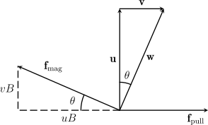
Two forces are applied to charge in vertical wire being pulled sideways. The electromotive force calculate the vertical component of magnetic force per unit charge \(\mathbf{f}_{\rm mag}\) at an instant: \[ \mathbf{f}_{\rm mag}\vdot \dd{\mathbf{l}} = vB\dd{\ell} \] where \(\dd{\mathbf{l}} = \mathbf{u} \dd{t}\). But the work is done by \(\mathbf{f}_{\rm pull}\): \[ \mathbf{f}_{\rm pull}\vdot \mathbf{w} \dd{t} = (uB) \frac{\dd{\ell}}{\cos\theta}\sin\theta = vB\dd{\ell} \]

For a freely moving closed wire under magnetic field: \[ \mathcal{E} = - \dv{\Phi}{t}. \]

The proportionality constant between the current in one loop and the magnetic flux through another loop: \[ \Phi_2 = M_{21}I_1. \]

The inductance on the loop itself.

The first equation:

The fourth equation:

Using Electromagnetic Tensor,

The first equation is also given by: \[ \partial_{[\alpha} F_{\beta\gamma]} = \partial_{\alpha} F_{\beta\gamma} + \partial_{\beta}F_{\gamma\alpha} + \partial_{\gamma}F_{\alpha\beta} = 0. \]

Using tensors, \[ \partial_{\mu}\partial^{\mu}A^{\nu} - \partial_{\mu}\partial^{\nu}A^{\mu} = \mu_0J^{\nu}. \]

In Lorenz gauge, \(\partial_{\mu}A^{\mu} = 0\), simplifying it to \[ \partial_{\mu}\partial^{\mu}A^{\nu} = \mu_0 J^{\nu}, \] which expands as:

This is in the form of inhomogeneous wave equation, and \(\rho, \mathbf{J}\) become the source terms.

\[ \pdv{\rho}{t} = - \div{\mathbf{J}}. \]

Using 4-current, \[ \partial_{\mu} J^{\mu} = 0. \]

• Poynting's Theorem

Work \(W\) done by electromagnetic field is given by:

The energy density \(u\) in electromagnetic field: \[ u := \frac{1}{2} \left( \varepsilon_0 E^2 + \frac{1}{\mu_0}B^2\right), \] and the Poynting vector \(\mathbf{S}\) that represent the energy flux (density) can be defined: \[ \mathbf{S} := \frac{1}{\mu_0} \mathbf{E}\cross \mathbf{B}. \]

When no work is done on the charges: \[ \pdv{u}{t} = - \div{\mathbf{S}} \] where \(u\) is the energy density in the first term.

Force exerted by electromagnetic field is given by:

The momentum density \(\mathbf{g}\): \[ \mathbf{g} := \mu_0\varepsilon_0 \mathbf{S} = \varepsilon_0 \mathbf{E}\cross \mathbf{B} \] and the electromagnetic stress or negative momentum flux (density) called Maxwell stress tensor \(\mathbf{T} = T^{ij}\mathbf{e}_i\otimes\mathbf{e}_j\) can be defined: \[ T^{ij} = \varepsilon_0 \left( E^iE^j - \frac{1}{2}\delta^{ij} E^2\right) + \frac{1}{\mu_0} \left( B^iB^j - \frac{1}{2} \delta^{ij} B^2 \right). \]

Total momentum of localized static field can be given in multiple equivalent forms:

where \(\mathbf{A}_{\rm C}\) is the vector potential in Coulomb gauge.

Naturally, electromagnetic field has angular momentum: \[ \vb*{\ell} = \mathbf{r}\cross \mathbf{g}. \]

\[ K^{\mu} = q u_{\nu} F^{\mu\nu} \] where \(u_{\mu}\) is the 4-velocity of the point charge.

The frame force of it is given by Lorentz force.

In a dynamic system, the potential changes as the charge distribution changes:

where \(t_{r} = t - |\mathbf{r} - \mathbf{r}'|/c\) is called the retarded time. These potentials satisfy the Lorenz gauge and its inhomogeneous wave equation.

The electric field and magnetic field can be obtained from the potential. When the retarded potential is substituted in, Jefimenko's equations are obtained, which help us calculate the fields from the charge and current, possibly easier:

This is the potential for a moving point charge. The charge appears to be different by the factor \((1 - (\widehat{\mathbf{r}- \mathbf{r}'})\vdot \mathbf{v} / c)^{-1}\).

The apparant elongation can be calculated from the difference in time it takes to arrive from the head and the tail of the object: \[ \frac{L'\cos\theta}{c} = \frac{L' - L}{v} \implies L' = \frac{L}{1 - v\cos\theta / c} \] where \(\theta\) is the angle between the velocity and the observer.

Given the trajectory of point charge \(\mathbf{w}(t)\),

where \(\mathbf{v} = \dot{\mathbf{w}}\), and \(t_r\) is given by the implicit equation \[ | \mathbf{r} - \mathbf{w}(t_r) | = c(t- t_r) \] with only one solution for each \(\mathbf{r}\), because the worldline of the point charge can only cross the light cone once.

From this potential, the fields can be calculated:

where \(\mathbf{u} := c(\widehat{\mathbf{r} - \mathbf{w}(t_r)}) - \mathbf{v}(t_r)\).

The first term decay as inverse square of distance and does not depend on the acceleration of the charge, and it is called generalized Coulomb field, or velocity field. The second term decay as inverse of distance and is called radiation field, or acceleration field.

The radiative power of point charge with zero velocity and acceleration \(a\) can be calculated from radiative field term, and given in Larmor formula: \[ \expval{P} = \frac{\mu_0 q^2 a^2}{6\pi c}. \] In general, with point charge with velocity, the radiative power is given by Liénard's generalization: \[ P = \frac{\mu_0q^2\gamma^6}{6\pi c} \left( a^2 - \left| \frac{\mathbf{v}\times \mathbf{a}}{c} \right|^2 \right). \] where \(\gamma\) is the gamma factor in relativity.

Given a electric dipole with charge concentrated at both ends and oscillates: \[ \mathbf{p}(t) = q_0 d\cos(\omega t) \vu{z} = p_0 \cos\theta \vu{z}, \] the retarded potential is given by

Using the approximation at the radiative zone \(d \ll \lambda \ll r\):

and the fields becomes:

The average radiative power of dipole radiation is then: \[ \expval{P} = \frac{\mu_0p_0^2\omega^4}{12\pi c}. \]

Given a magnetic dipole of small circular circuit with oscillating current: \[ \mathbf{m}(t) = \pi b^2 I_0 \cos\theta \vu{z} = m_0 \cos\theta \vu{z}, \] the same procedure with radiative zone approximation \(d \ll \lambda \ll r\), almost identical result is obtained:

with radiative power of \[ \expval{P} = \frac{\mu_0m_0^2\omega^4}{12\pi c^3}. \]

The radiative power is tiny compared to electric dipole \[ \frac{P_{\rm magnetic}}{P_{\rm electric}} = \left( \frac{m_0}{p_0 c} \right)^2 = \left( \frac{\omega b}{c} \right)^2. \]

The charge experience recoil force by the emitted field, From the average energy emitted by charge:

Abraham-Lorentz formula is inspired by this: \[ \mathbf{F}_{\rm rad} = \frac{\mu_0q^2}{6 \pi c} \dot{\mathbf{a}}. \] This formula has to be used with care, because one solution to this is exponential growth.

Reaction force arises from the first order time-derivative of acceleration term of self-force, which charge exerts on itself retardedly.

\[ \gamma := \frac{q}{2m} \]

\[ \gamma_{\rm e} := \frac{-e}{2m_{\rm e}}|g_{\rm e}| = \frac{g_{\rm e}\mu_{\rm B}}{\hbar} \] It deviate from the classical result by the g-factor.

\[ \gamma = \frac{e}{2m_{\rm p}}g_{\rm n} = \frac{g_{\rm n}\mu_{\rm N}}{\hbar} \]