Metrology
Table of Contents
- 1. Commensurable
- 2. Conversion Factor
- 3. Common Units
- 4. Centimeter-Gram-Second System of Units
- 5. Radiometry and Photometry
- 6. Dosimetry
- 7. Natural Units
- 8. Obscure Units
- 9. See Also
- 10. Reference
There is no unit in mathematics in the first place. By assigning units to quantities, you are endowing the quantity a physical significance. Therefore the physicality has to be taken into account thereon.
1. Commensurable
- Two units are commensurable if they can added together.
2. Conversion Factor
- A dimensionless number 1 that is a ratio of two measures.
- e.g. \(1=100\, \mathrm{cm}/1\,\mathrm{m}\)
- For incommensurable units, it depends on the context.
- e.g. \(1=100\, \mathrm{km}/3\,\mathrm{h}\iff 100 \mathrm{km}=3\,\mathrm{h}\)
- Degree, the unit of angle, can be thought of as a conversion factor.
- \[^{\circ} =\frac{\pi}{180}\]
3. Common Units
3.1. SI Units
- International System of Quantities (ISQ)
3.1.1. SI Base Units
| Quantity | Quantity Symbol | Dimension | SI Base Unit |
|---|---|---|---|
| Length | \(l\) | \(\sf L\) | \(\rm m\) |
| Mass | \(m\) | \(\sf M\) | \(\rm kg\) |
| Time | \(t\) | \(\sf T\) | \(\rm s\) |
| Electric Current | \(I\) | \(\sf I\) | \(\rm A\) |
| Thermodynamic Temperature | \(T\) | \(\sf \Theta\) | \(\rm K\) |
| Amount of Substance | \(n\) | \(\sf N\) | \(\rm mol\) |
| Luminous Intensity | \(I_\mathrm{v}\) | \(\sf J\) | \(\rm cd\) |
3.1.2. SI Derived Units
| Name | Symbol |
|---|---|
| radian | \(\rm rad\) |
| steradian | \(\rm sr\) |
| hertz | \(\rm Hz\) |
| newton | \(\rm N\) |
| pascal | \(\rm Pa\) |
| joule | \(\rm J\) |
| watt | \(\rm W\) |
| coulomb | \(\rm C\) |
| volt | \(\rm V\) |
| farad | \(\rm F\) |
| ohm | \(\Omega\) |
| siemens | \(\rm S\) |
| weber | \(\rm Wb\) |
| tesla | \(\rm T\) |
| henry | \(\rm H\) |
| degree Celsius | \(\rm ^\circ C\) |
| lumen | \(\rm lm\) |
| lux | \(\rm lx\) |
| becquerel | \(\rm Bq\) |
| gray | \(\rm Gy\) |
| sievert | \(\rm Sv\) |
| katal | \(\rm kat\) |
| Unit | |
|---|---|
| Electric Field | \(\rm V/m\) |
| Permittivity | \(\rm F/m\) |
3.1.3. Prefixes
| Name | Symbol | Base 10 Factor |
|---|---|---|
| quetta | \(\rm Q\) | \(10^{30}\) |
| ronna | \(\rm R\) | \(10^{27}\) |
| yotta | \(\rm Y\) | \(10^{24}\) |
| zetta | \(\rm Z\) | \(10^{21}\) |
| exa | \(\rm E\) | \(10^{18}\) |
| peta | \(\rm P\) | \(10^{15}\) |
| tera | \(\rm T\) | \(10^{12}\) |
| giga | \(\rm G\) | \(10^{9}\) |
| mega | \(\rm M\) | \(10^{6}\) |
| kilo | \(\rm k\) | \(10^3\) |
| hecto | \(\rm h\) | \(10^2\) |
| deca | \(\rm da\) | \(10^1\) |
| \(\text{--}\) | \(\text{--}\) | \(1\) |
| deci | \(\rm d\) | \(10^{-1}\) |
| centi | \(\rm c\) | \(10^{-2}\) |
| milli | \(\rm m\) | \(10^{-3}\) |
| micro | μ | \(10^{-6}\) |
| nano | \(\rm n\) | \(10^{-9}\) |
| pico | \(\rm p\) | \(10^{-12}\) |
| femto | \(\rm f\) | \(10^{-15}\) |
| atto | \(\rm a\) | \(10^{-18}\) |
| zepto | \(\rm z\) | \(10^{-21}\) |
| yocto | \(\rm y\) | \(10^{-24}\) |
| ronto | \(\rm r\) | \(10^{-27}\) |
| quecto | \(\rm q\) | \(10^{-30}\) |
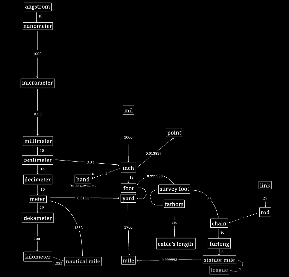
3.2. Avoirdupois
- a defense of the imperial measurement system - YouTube
- Imperial Units
- US Customary Units
- Yard-Pound System
- Everyday use in USA1
3.2.1. Length
Yard
- 0.9144 m
- 3 feet
Mile
- 1760 yards.
- It originated from the different unit system, the Roman one.
3.2.2. Weight
Pound
- 0.454 kg
Ounce
- oz, oz.
- Alchemical symbol for an ounce ℥, and half an ounce 🝳.
- 28.34 g
3.2.3. Volume
Fluid Ounce
- fl oz, fl. oz.
- US Customary: 29.57 mL
- US Food Labelling: 30 mL
Gill
- 4 US fluid ounces
- 5 imperial fluid ounces
Pint
- 4 gills
Quart
- quarter gallon
- 2 pints
Gallon
- gal
- US Gallon: 231 in³ (≈ 3.785 L)
- 4 quarts
3.2.4. Point
- The definition may vary.
3.2.4.1. DTP
- desktop publishing point
- 1/72 of an inch, 1/12 of a pica.
- 0.3528 mm.
3.2.4.2. New Didot Point
nd- 3/8 mm, or 0.375 mm.
3.2.4.3. American Point
- American point system
- 1/72.27 of an inch,
- TeX point 0.351 459 80 mm
- Point (typography) - Wikipedia
3.2.5. Horsepower
- Watt determined that a horse could turn a mill wheel 144 times in an hour, or 2.4 times in a minute. The wheel was 12 feet (3.7 m) in radius, and Watt judged that the horse could pull with a force of 180 pounds-force (800 N).
- \[ 1\,\mathrm{hp} = 180\,\mathrm{lbf}\cdot 2.4\,\mathrm{turn/min}\cdot (2\pi\cdot 12)\,\mathrm{ft/turn} = 32,572\,\mathrm{ft\,lbf/min} \]
3.2.5.1. Imperial Horsepower
- \(1\,\mathrm{hp} = 745.7\,\mathrm{W}\)
3.2.5.2. Metric Horsepower
- 735.5 W
3.3. Level
3.3.1. Decibel
- dB (base quantity) is the unit of the level.
\[ L = 10 \log \frac{Q}{Q_0}\ \mathrm{dB} \]
- A reference unit can be provided so that the quantity have a unit.
3.3.1.1. dBm
- decibel-milliwatts
3.3.1.2. Root-Power Quantity
- Often used for voltage.
- 20 is used.
3.3.2. Neper
- Np
- natural logarithm is used.
3.4. Information
3.4.1. Shannon
- Log 2 of probability
3.4.2. Nat
- Natural log of probability
4. Centimeter-Gram-Second System of Units
- CGS Units, CGS, cgs
| Quantity | Quantity Symbol | Unit Name | Unit Symbol | Description |
|---|---|---|---|---|
| Acceleration | \(a\) | gal(galileo) | \(\rm Gal\) | |
| Force | \(F\) | dyne | \(\rm dyn\) | From Greek, δύναμις, "power" |
| Energy | \(E\) | erg | \(\rm erg\) | From Greek, ἔργον, "work" |
| Pressure | \(p\) | barye | \(\rm Ba\) | |
| Dynamic Viscosity | \(\mu\) | poise | \(\rm P\) | \(\rm cP\) is more common |
| Kinematic Viscosity | \(\nu\) | stokes | \(\rm St\) | |
| Wavenumber | \(k\) | kayser | \(\rm K\) |
For electromagnetic CGS units, we do not invent new units but simply measure it indirectly in conventional units.
4.1. Electrostatic Units
- ESU, CGS-ESU
4.1.1. Statcoulomb
- \(\rm statC\), \(\rm Fr\)
- , esu charge
Electrostatic units first define the unit of charge, and derive other units from it.
It is defined by the Coulomb's law: \[ \mathbf{F} = \frac{q_1^\mathsf{ESU}q_2^\mathsf{ESU}}{r^2} \vu{r}. \] The unit of charge is called statcoulomb, and it is the amount of charge that exert one dyne of force when one centimeter apart from the same charge: \[ \rm statC = \sqrt{dyn \cdot cm^2} = cm^{3/2}\cdot g^{1/2}\cdot s^{-1} \] The point is to express charge entirely from mass, length, and time.
Statcoulomb is related to the SI unit coulomb by 1 C ≘ 10⁻¹ c statC, and the dimensions are related by: \[ q^\mathsf{ESU} = \frac{q^\mathsf{I}}{\sqrt{4\pi\varepsilon_0}} \]
Statcoulomb is related to the electromagnetic unit abcoulomb by c statC ≘ 1 abC, and the dimensions are also related by: \[ q^{\mathsf{ESU}} = c q^{\mathsf{EMU}}. \]
The factor of \(c\) between these units stayed mystery until the unification of electricity and magnetism.
4.1.2. Statampere
\[ \rm statA := \frac{statC}{s} = cm^{3/2}\cdot g^{1/2} \cdot s^{-2} = \sqrt{dyn} \cdot cm \cdot s^{-1} \]
4.1.3. Statvolt
\[ \rm statV := \frac{erg}{statC} = \frac{cm^2\cdot g\cdot s^{-2}}{cm^{3/2}\cdot g^{1/2}\cdot s^{-1}} = cm^{1/2}\cdot g^{1/2}\cdot s^{-1} = \sqrt{dyn} \]
4.1.4. Statvolt per Centimeter
\[ \rm statV \cdot cm^{-1} = \sqrt{dyn} \cdot cm^{-1} \]
The unit of electric filed is defined by the definition of electric field: \[ \mathbf{E}^\mathsf{ESU} = \frac{q^\mathsf{ESU}}{r^2}\mathbf{\hat{r}} = \frac{\mathbf{F}}{q^\mathsf{ESU}}. \]
The relation to the SI system is: \[ \mathbf{E}^\mathsf{ESU} = \sqrt{4\pi\varepsilon_0}\,\mathbf{E}^\mathsf{SI} \]
4.1.5. Statohm
\[ \rm stat \text{\Omega} := \frac{statV}{statA} = cm^{-1}\cdot s \]
4.1.6. Stattesla
- \(\rm statT\)
It is defined by the Lorentz force: \[ \mathbf{F} = q^{\sf ESU}\mathbf{v}\times \mathbf{B}^{\sf ESU}. \]
\[ \rm statT := \frac{dyn\cdot s}{statC\cdot cm} = cm^{-3/2}\cdot g^{1/2} = \sqrt{dyn} \cdot s \cdot cm^{-2} \]
Stattesla is related to the SI unit tesla by 1T ≘ 10⁻⁴ c⁻¹ statT, and the dimensions are related by: \[ \mathbf{B}^{\sf ESU} = \sqrt{4\pi\varepsilon_0}\,\mathbf{B}^{\sf SI} = \sqrt{\frac{4\pi}{\mu_0}}\frac{\mathbf{B}^{\mathsf{SI}}}{c}. \]
It does not include the factor of \(c\), compared to Gauss.
4.1.7. Statweber
- The unit of magnetic flux
\[ \rm statWb := statT \cdot cm^2 \]
4.2. Electromagnetic Units
- EMU, CGS-EMU
4.2.1. Abampere
- \(\rm abA\), \(\rm Bi\)
- Biot, emu current
Electromagnetic units first define the unit of current, and derive other units from it.
It is defined by the force per centimeter \(f\) between two parallel wires of infinite length: \[ \frac{f}{2} =\frac{I_1^{\sf EMU}I_2^{\sf EMU}}{r}. \] The unit of current is called abampere, and it is the amount of current that exert two dyne per centimeter of force for two wires with same current are one centimeter apart from each other.
The factor of two is to cancel the two that arises for the magnetic field when applying the Biot-Savart law \[ \mathbf{B}^{\sf EMU} = \frac{I^{\sf EMU}\dd{\mathbf{l}}\times \mathbf{\hat{r}}}{r^2} \] for infinitely long wires, and applying the Lorentz force \[ \mathbf{F} = I^{\mathsf{EMU}} \dd{\mathbf{l}} \times \mathbf{B}^{\mathsf{EMU}}. \]
When represented with basis units: \[ \rm abA = \sqrt{dyn} = g^{1/2}\cdot cm^{1/2}\cdot s^{-1}. \]
Abampere is related to the SI unit ampere by 1 A ≘ 10⁻¹ abA and the dimensions are related by: \[ I^{\sf EMU} = \frac{I^{\sf SI}}{\sqrt{4\pi / \mu_0}} = \frac{I^{\sf SI}}{c\sqrt{4\pi\varepsilon_0}}. \]
4.2.2. Abcoulomb
\[ \rm abC := abA \cdot s = g^{1/2}\cdot cm^{1/2} = \sqrt{dyn} \cdot s \]
4.2.3. Gauss
- Abtesla
Gauss is defined to be consistent with Biot-Savart law and Lorentz force, as explained above in abampere. \[ \rm G = \frac{dyn}{abA \cdot cm} = \frac{abA \cdot cm}{cm^2} = cm^{-1/2}\cdot g^{1/2}\cdot s^{-1} = \sqrt{dyn}\cdot cm^{-1} \]
The relation to the SI unit tesla is: 1 T ≘ 10⁴ G and the dimensions are related by: \[ \mathbf{B}^{\sf EMU} = c\sqrt{4\pi\varepsilon_0}\,\mathbf{B}^{\sf SI} = \sqrt{4\pi/\mu_0}\mathbf{B}^{\mathsf{SI}}. \]
It is related to the electrostatic unit stattesla by: 1 statT ≘ c G while the dimensions are related by: \[ c\mathbf{B}^{\mathsf{ESU}} = \mathbf{B}^{\mathsf{EMU}}. \]
The conversion factor \(10^4\) from gauss to tesla is particularly nice due to the value of permeability of the vacuum. \[ \frac{B^{\mathsf{EMU}}}{B^\mathsf{SI}} = \sqrt{\frac{4\pi}{\mu_0}} \approx \sqrt{\frac{4\pi}{4\pi\times 10^{-7}\ \mathrm{N/A^2}}} = 10^{\frac{7}{2}}\rm\ N^{-1/2}A = \frac{10^4\ G}{1\ T} \]
The digits of permeability of vacuum being so close to \(4\pi\) is in fact not a coincidence. Because the early definition (until 2019) of the unit of magnetic field was:
- 1/(2⋅10⁻⁷) times
- the magnetic field strength produced at one of the two identical infinitely long wire
- with identical electric current flowing
- separated by one meter
- and exert force of 2⋅10⁻⁷ neuton per meter to each other (definition of 1 ampere).
Just like the defintiion of Gauss.
In order to cancel the inclusion of \(4\pi\) in the denominator of Biot-Savart law, \(4\pi\) is included in \(\mu_0\), and in order to reduce the effect of infinite wire to a infinitesimal segment, the force is halved, giving us the final formula for the familiar Biot-Savar law: \[ \mathbf{B} = \frac{\mu_0}{4\pi} \frac{I \dd{\mathbf{l}}\times \vu{\mathbf{r}}}{r^2} \] and the value of permeability of vacuum: \[ \mu_0 = 4\pi \times 10^{-7}\,\rm T\cdot m/A. \]
After 2019, ampere has been decoupled from the unit of force, and how much force it generates is now a matter of measurement.
4.2.4. Oersted
The unit of auxiliary magnetic field \(\mathbf{H}\) \[ \rm Oe := abA \cdot cm^{-1} \]
4.2.5. Maxwell
The unit of magnetic flux \(\Phi\) \[ \rm Mx := G \cdot cm^2 \]
4.3. Gaussian Units
- CGS-Gaussian
- Gaussian Unit System, Gaussian-CGS Units, CGS Units
Gaussian unit system follows ESU for electricity and EMU for magnetism. It choose Gauss for its unit of magnetic field, hence the name.
| Quantity | ESU | EMU |
|---|---|---|
| Electric Charge | Franklin | |
| Electric Current | statA | |
| Electric Potential | statV | |
| Electric Field | statV/cm | |
| Electric Displacement Filed | statC/cm² | |
| Electric Dipole Moment | statC⋅cm | |
| Permittivity | 4π⋅10¹¹⋅(c⋅s/cm)² | |
| Resistance | statΩ | |
| Magnetic B Field | Gauss | |
| Magnetic H Field | Oersted | |
| Magnetic Dipole Moment | erg/G | |
| Magnetic Flux | Maxwell | |
| Permeability | 10⁷/4π |
Since two systems do not agree in its dimension, the equations related to electromagnetism are adjusted accordingly. Due to the fact that electric field and magnetic field having same dimension, the equations tends to simplify: Lorentz Force \[ \mathbf{F} = q^\mathrm{\mathsf{G}}\left(\mathbf{E}^\mathrm{\mathsf{G}} + \frac{1}{c}\mathbf{v}\times \mathbf{B}^\mathrm{\mathsf{G}}\right) \]
Maxwell's Equations \[ \nabla\cdot \mathbf{E}^\mathsf{G} = 4\pi \rho^\mathsf{G} \] \[ \nabla \cdot \mathbf{B}^\mathsf{G} = 0 \] \[ \nabla\times \mathbf{E}^\mathsf{G} + \frac{1}{c} \frac{\partial \mathbf{B}^\mathsf{G}}{\partial t} = 0 \] \[ \nabla\times \mathbf{B}^\mathsf{G} - \frac{1}{c}\frac{\partial \mathbf{E}^\mathsf{G}}{\partial t} = \frac{4\pi}{c}\mathbf{J}^\mathsf{G} \]
5. Radiometry and Photometry
Radiometry deals with raw electromagnetic radiation while photometry deals with how they are perceived. Radiometry uses subscript \(\rm e\) for "energetic" and photometry uses subscript \(\rm v\) to avoid confusion.
5.1. Radiant Flux
- Radiant Power, Luminosity (in astronomy)
- \(\rm W\)
- Radiant energy emitted, reflected, transmitted, or received per unit time.
\[ \Phi_{\rm e} := \dv{Q_{\rm e}}{t} \] where \(Q_{\rm e}\) is the radiant energy passing a closed surface \(\Sigma\) in time interval \(T\): \[ Q_{\rm e} := \int_T\in_{\Sigma} \mathbf{S} \vdot \vu{n} \dd{A}\dd{t}. \]
Radiant flux can be either the average flux or the instantaneous flux.
5.2. Radiant Intensity
- \(\rm W/sr\)
- Radiant flux emitted, reflected, transmitted, or received per unit solid angle.
\[ I_{\rm e, \Omega} := \pdv{\Phi_{\rm e}}{\Omega} \]
5.2.1. Spectral Intensity
Spectral intensity in frequency \[ I_{\rm e, \Omega, \nu} := \pdv{I_{\rm e, \Omega}}{\nu} \]
Spectral intensity in frequency \[ I_{\rm e, \Omega, \lambda} := \pdv{I_{\rm e, \omega}}{\lambda} \]
5.3. Irradiance
- \(\rm W/m^2\)
- Radiant flux received by a surface per unit area.
\[ E_{\rm e} := \pdv{\Phi_{\rm e}}{A} \]
5.3.1. Spectral Irradiance
Spectral irradiance in frequency \[ E_{\rm e, \nu} := \pdv{E_{\rm e}}{\nu} \]
Spectral irradiance in wavelength \[ E_{\rm e, \lambda} := \pdv{E_{\rm e}}{\lambda} \]
5.4. Radiant Exposure
- Fluence
Radiant energy received by a surface per unit area.
\[ H_{\rm e} := \pdv{Q_{\rm e}}{A} = \int_0^T E_{\rm e}(t)\dd{t} \] where \(T\) is the duration of irradiation.
5.4.1. Spectral Irradiance
Spectral exposure in frequency \[ H_{\rm e, \nu} := \pdv{H_{\rm e}}{\nu} \]
Spectral irradiance in wavelength \[ H_{\rm e, \lambda} := \pdv{H_{\rm e}}{\lambda} \]
5.5. Radiant Exitance
- Radiant Emittance
- \(\rm W/m^2\)
- Radiant flux emitted by a surface per unit area.
\[ M_{\rm e} := \pdv{\Phi_{\rm e}}{A} \]
5.5.1. Spectral Exitance
Spectral exitance in frequency \[ M_{\rm e, \nu} := \pdv{M_{\rm e}}{\nu} \]
Spectral exitance in wavelength \[ M_{\rm e, \lambda} := \pdv{M_{\rm e}}{\lambda} \]
5.6. Radiosity
- Radiant flux leaving (emitted, reflected, and transmitted by) a surface per unit area.
\[ J_{\rm e} := \pdv{\Phi_{\rm e}}{A} = J_{\rm e, em} + J_{\rm e, r} + J_{\rm e, tr} \] where \(J_{\rm e,em} = M_{\rm e}\) is the radiant exitance, \(J_{\rm e,r}\) is the reflected component, and \(J_{\rm e, tr}\) is the transmitted component.
5.6.1. Spectral Radiosity
Spectral radiosity in frequency \[ J_{\rm e, \nu} := \pdv{J_{\rm e}}{\nu} \]
Spectral radiosity in wavelength \[ J_{\rm e, \lambda} := \pdv{J_{\rm e}}{\lambda} \]
5.7. Radiance
- Historically, "intensity" in heat transfer, astrophysics and astronomy
Radiant flux emitted, reflected, transmitted or received by a given surface, per unit solid angle per unit projected area.
\[ L_{\rm e, \Omega} := \frac{\partial^2\Phi_{\rm e}}{\partial\Omega\partial (A\cos\theta)} \] where \(\Omega\) is the solid angle, \(A\cos\theta\) is the projected area.
5.7.1. Spectral Radiance
Spectral radiance in frequency \[ L_{\rm e, \Omega,\nu} := \pdv{L_{\rm e, \Omega}}{\nu} \]
Spectral radiance in wavelength \[ L_{\rm e, \Omega, \lambda} := \pdv{L_{\rm e, \Omega}}{\lambda} \]
5.8. Luminous Efficacy
- \(\rm lm/W\)
- The efficiency of producing visible light.
Ratio of luminous flux to power. The power can be either the radiant flux of the source's output, or the total power (electric, chemical, or others) consumed by the source. The former sense is sometimes called the luminous efficacy of radiation \(K\), and the latter luminous efficacy of a light source \(\eta\) or overall luminous efficacy.
\[ K = \frac{\Phi_{\rm v}}{\Phi_{\rm e}} = \frac{\int_0^{\infty} K(\lambda) \Phi_{\rm e, \lambda}\dd{\lambda}}{\Phi_{\rm e, \lambda}\dd{\lambda}} \] where \(K(\lambda) = K_{\rm m} \bar{y}(\lambda)\) is the spectral luminous efficacy, consisting of maximum spectral luminous efficacy \(K_{\rm m} = 683.002\, \mathrm{lm/W}\) and luminous efficiency function defined by CIE.
5.9. Luminous Flux
- Luminous Power
Perceived power of light
lumen \(\rm lm\) Luminous flux of light produced by a light source that emits one candela of luminous intensity over a solid angle of one steradian.
\[ 1\, \mathrm{lm} = 1\, \mathrm{cd} \cdot 1 \, \mathrm{sr}. \]
It is wavelength-weighted power by the luminous efficiency function \(\bar{y}(\lambda)\) (sometimes \(V(\lambda)\)): \[ \Phi_{\rm v} = (683.002\, \mathrm{lm/W}) \int_0^{\infty} \bar{y}(\lambda) \Phi_{\rm e, \lambda} (\lambda) \dd{\lambda} \] where \(\Phi_{\rm e, \lambda}\) is the spectral radiant flux.
5.10. Luminous Intensity
Perceived power of light per solid angle.
candela \(\rm cd\) SI Base Units
5.11. Illuminance
Total luminous flux incident on a surface per unit area.
lux \(\rm lx\)
5.12. Luminous Exposure
- \(\rm lx\cdot s\)
\[ H_{\rm v} := \int_0^T E_{\rm v}(t)\dd{t} \]
5.13. Luminous Exitance
- Luminous Emittance
Luminous flux emitted from a surface per unit area
5.14. Luminance
Luminous intensity per unit area.
\[ L_{\rm v} = \frac{\dd[2]\Phi_{\rm v}}{\dd{\Sigma}\dd{\Omega_{\Sigma}}\cos\theta_{\Sigma}} \] where \(\dd[2]{\Phi_{\rm v}}\) is the luminous flux leaving the area \(\dd{\Sigma}\) in any direction contained inside the solid angle \(\dd{\Omega}_{\Sigma}\), \(\dd{\Sigma}\) is an infinitesimal area of the source, \(\dd{\Omega_{\Sigma}}\) is an infinitesimal solid angle containing the specified direction, \(\theta_{\Sigma}\) is the angle between the normal \(\vu{n}_{\Sigma}\) to the surface \(\dd{\Sigma}\) and the specified direction.
In a lossless medium, the luminance does not change along a given light ray. For an arbitrary surface \(S\) being illuminated, the luminance is given by: \[ L_{\rm v} = \frac{\dd[2]\Phi_{\rm v}}{\dd{S}\dd{\Omega_{S}}\cos\theta_{S}} \] where \(\dd{S}\) is the infinitesimal area of \(S\) seem from the source inside the solid angle \(\dd{\Omega_{\Sigma}}\), \(\dd{\Omega_S}\) is the infinitesimal solid angle subteded by \(\dd{\Sigma}\) as seen from \(\dd{S}\), \(\theta_S\) is the angle between the normal \(\vu{n}_S\) to \(\dd{S}\) and the direction of the light.
More generally, the luminance along a light ray is defined as: \[ L_{\rm v} = n^2 \dv{\Phi_{\rm v}}{G} \] where \(\dd{G}\) is the etendue of an infinitesimally narrow beam containing the specified ray, \( \dd{\Phi_{\rm v}} \) is the luminous flux carried by this beam, and \(n\) is the index of refraction of the medium.
nit
- \(\rm nt\), \(\rm cd/m^2\)
- The name probably come from Latin nitēre "to shine".
stilb
- \(\rm sb\), \(\rm cd/cm^2\)
- CGS unit
lambert
- \(1/\pi\) candela per square centimeter
apostilb, bril, skot are obsolete units
6. Dosimetry
6.1. Activity
Number of radioactive transformations per second on average.
Becquerel \(\rm Bq\) One decay per second.
Curie \(\rm Ci\) Originally the quantity or mass of radium emanation in equilibrium with one gram of radium, but now redefined as \[ 1\, \rm Ci = 3.7\times 10^{10}\, \text{decay/s}. \]
Rutherford \(\rm Rd\)
6.2. Radiation Exposure
- \(\rm C/kg\)
Ionization of air due to ionizing radiation from photons, measured in electric charge freed by such radiation within a region of air divided by the mass of that air.
6.3. Absorbed Dose
- \(\rm Gy = J/kg\)
Energy per unit mass (specific energy) deposited by ionizing radiation.
6.4. Equivalent Dose
- \(\rm Sv\)
\[ H_T := \sum_R W_R D_{T,R} \] where \(W_R\) is the radiation weighting factor defined by regulation, \(D_{T,R}\) is the absorbed dose in tissue \(T\) by radiation type \(R\),
6.5. Effective Dose
- \(\rm Sv\)
where \(E\) is the effective dose to the entire organism, \(H_T\) is the equivalent dose absorbed by tissue \(T\), \(W_T\) is the tissue weighting factor defined by regulation, \(W_R\) is the radiation weighting factor defined by regulation, \(\bar{D}_{T,R}\) is the mass-averaged absorbed dose in tissue \(T\) by radiation type \(R\), \(D_R(\mathbf{x})\) is the absorbed dose from radiation type \(R\) as a function of location, \(\rho(\mathbf{x})\) is the density as a function of location, \(V\) is volume, and \(T\) is the tissue or organ of interest.
6.6. Dose Equivalent
- Operational Quantity
7. Natural Units
7.1. Planck Units
7.1.1. Quantities
- Every quantities are scaled by the factor of plank quantities, yielding dimensionless quantities that corresponds to the normal quantities.
| Name | Expression |
|---|---|
| Plank length | \(l_\text{P} = \sqrt{\dfrac{\hbar G}{c^3}}\) |
| Plank mass | \(m_\text{P} = \sqrt{\dfrac{\hbar c}{G}}\) |
| Plank time | \(t_\text{P} = \sqrt{\dfrac{\hbar G}{c^5}}\) |
| Plank temperature | \(T_\text{P} = \sqrt{\dfrac{\hbar c^5}{Gk_\text{B}^2}}\) |
| Plank charge | \(q_\text{P} = \sqrt{4\pi\varepsilon_0\hbar c}\ (k_\text{B} = 1)\quad\text{or}\quad \sqrt{\varepsilon_0\hbar c}\ (\varepsilon_0 = 1)\) |
7.1.2. Units
- The units can be thought of as the ratio to the Plank quantities.
- e.g.
- \[ [\text{length}] = \frac{\rm m}{l_\text{P}} \]
- e.g.
7.1.3. Implications
- The effect is equivalent to setting \(c = G = \hbar = k_\text{B} = 1\)
- \[ F = \frac{m_1m_2}{r^2} \]
7.2. Heaviside-Lorentz Units
7.2.1. Quantities
- Only the \(\varepsilon_0\) is removed compared to the Gaussian units.
- \[ q^{\sf HL} := \frac{q^{\sf SI}}{\sqrt{\varepsilon_0}} \]
- \[ \mathbf{E}^{\sf HL} := \sqrt{\varepsilon_0}\,\mathbf{E}^{\sf SI} \]
- \[ \mathbf{B}^{\sf HL} := c\sqrt{\varepsilon_0}\,\mathbf{B}^{\sf SI} = \frac{1}{\sqrt{\mu_0}}\mathbf{B}^{\sf SI} \]
7.3. Atomic Units
7.3.1. Quantities
- Similar to Planck units, but set \(\hbar = e = m_\text{e} = 4\pi\varepsilon_0 = 1\).
8. Obscure Units
8.1. Airwatt
\( \rm AW, airW \)
The product of suction pressure (in Pascal) and air flow rate (in cubic meter per second): \[ P = p\cdot Q. \]
9. See Also
- How To Multiply Dog × Tree?! A Dimensional Analysis Primer - YouTube: Anything is unit
- Cursed Units 2: Curseder Units - YouTube
- Radian
- \[ \rm rad = \frac{arclength}{radius} \]
- pH
- \[ \rm pH = -\log\left(\frac{molar\ concentration}{1\ mol/L}\right) \]
- Radian
- \(\stackrel{\frown}{=}\), ≘ U+2258
- 'Corresponds'
10. Reference
- International System of Units - Wikipedia
- International System of Quantities - Wikipedia
- SI derived unit - Wikipedia
- Gallon - Wikipedia
- Decibel - Wikipedia
- dBm - Wikipedia
- Shannon (unit) - Wikipedia
- International System of Units - Wikipedia
- International System of Quantities - Wikipedia
- SI derived unit - Wikipedia
- Centimetre–gram–second system of units - Wikipedia
- Gaussian units - Wikipedia
- Radiosity (radiometry) - Wikipedia
- Effective dose (radiation) - Wikipedia
- Planck units - Wikipedia
- Heaviside–Lorentz units - Wikipedia
- Atomic units - Wikipedia
- Airwatt - Wikipedia